By Pramodith B, Member of Technical Staff
Dense Matmuls are faster when the inputs are sparse
The code and raw results are available here.
Introduction
Dense matrices. A dense matrix is one where (almost) every entry is non-zero and every entry is stored explicitly in memory. A bf16 8192x8192 matrix takes 8192 x 8192 x 2 bytes = 128 MiB, whatever the values are. Neural-network weights and activations are almost always stored and multiplied this way.
Sparse matrices. A sparse matrix is one where many of the entries are zero. We call the fraction of zeros its sparsity: a matrix with 90% sparsity has nine zeros for every non-zero. Sparse matrices can be stored in compressed formats that keep only the non-zero values and their positions, or they can be stored densely, zeros and all. In LLMs, zeros come from pruning weights or from activation functions like ReLU, which output zero for every negative input.
How GPUs accelerate sparsity today. Multiplying by zero is wasted work, so in principle a sparse matmul should be cheaper. In practice, scattered zeros are hard for GPUs to exploit because they break the regular memory access and compute patterns that tensor cores depend on. NVIDIA’s answer, starting with Ampere and continuing in Hopper and Blackwell, is semi-structured (2:4) sparsity: in every group of four consecutive values, at most two are non-zero. A matrix that follows this pattern is stored compressed (the non-zero half of the values plus a small index per value saying where it came from), and the Sparse Tensor Cores run dedicated sparse matrix-multiply-accumulate instructions (mma.sp in PTX) that skip the zeros entirely. That gives up to twice the peak math throughput of a dense matmul (NVIDIA, Ampere Architecture In-Depth; Mishra et al., 2021). The catch is that you need a specialized kernel (cuSPARSELt, or PyTorch’s to_sparse_semi_structured) and the model has to be pruned to exactly that 2:4 pattern, which usually costs some accuracy.
What about plain dense kernels? A normal dense kernel knows nothing about zeros: it loads every value and does every multiply, so you would expect its runtime to be the same whatever the data. This post shows that it is not. Dense matmuls run up to 18% faster when one input is sparse, even with zeros stored densely, at random positions, and with no sparse kernel involved.
Experimental setup
x @ win bf16 withwof shape 8192x8192 andxof shapeM x 8192, run with plaintorch.matmul(cuBLAS). No sparse kernels are involved.- The fraction of
wset to zero is varied over 5%, 10%, 25%, 50%, 70%, 90% and 99%, with positions chosen uniformly at random; the measured zero fraction matches to within 2e-7 and is stored in the results. The activationsxare dense Gaussian. - Everything below is “speedup over the dense weight”, i.e. dense time divided by time with zeros, so values above 1.000 mean faster than dense.
- Matmuls are captured in a CUDA graph and timed over replays to minimize launch overhead. Each graph rotates through 8 independent copies of the weight, the activations and the output (each weight copy has its own random zero positions), so the same tensor is only touched again after at least a gigabyte of other traffic, far more than the L2 cache. Without this, the same 128 MiB weight would be re-read from cache on every replay. Every config is timed in 5 interleaved rounds (alternating order) and we report the median, so drift hits every config equally.
Mis swept over 1024, 2048, 4096, 8192 and 16384. In an exploratory run on the H100 with smallerM(1, 16 and 128 rows) the matmul is memory-bound and sparsity made no difference (within 0.5%), so we start this sweep at 1024. We come back to why smallMshows no effect in the inference section.- We use one H100 80GB HBM3 (700 W power limit) and one B200 (1000 W power limit). Alongside each timing we log the SM clock and board power from NVML.
Results: speedup at different sparsity levels
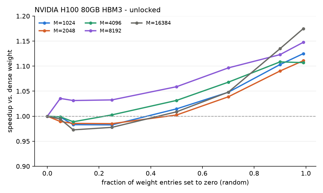
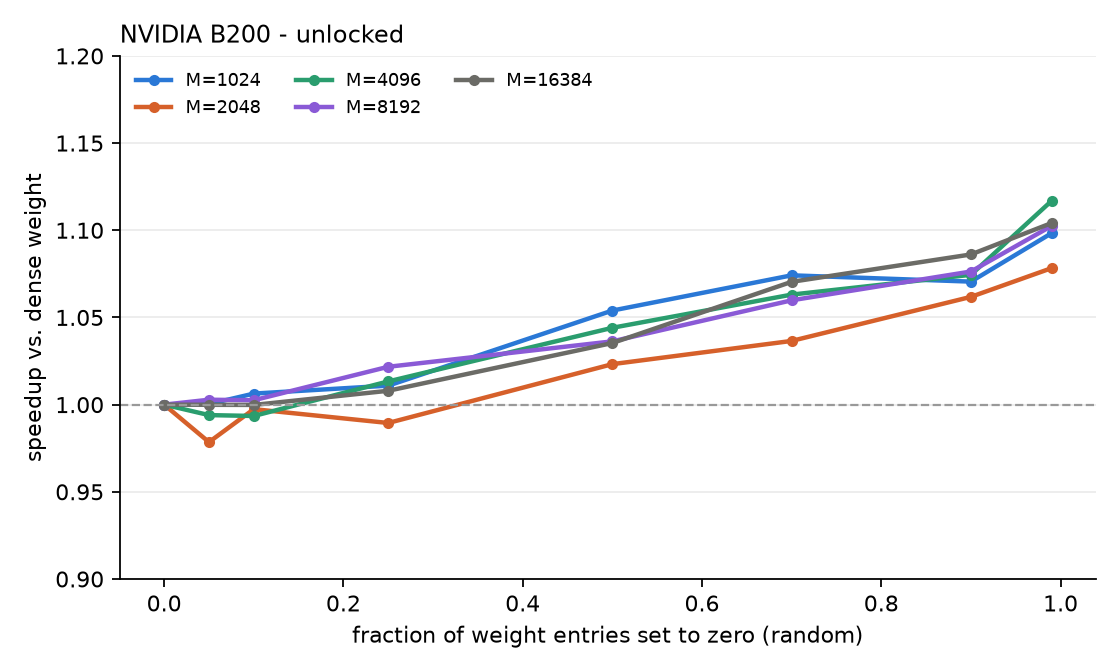
- Speedup grows with the amount of zeros, up to about 1.18x on the H100 and 1.12x on the B200.
- It takes a lot of zeros to matter. At 50% zeros the speedup is 1.00-1.06x, and at 5-25% it is mostly inside the run-to-run noise. On the H100, 5-25% zeros was up to 2% slower than dense for several shapes.
The clock and power samples show where the speedup comes from. Dense and 99%-zero runs draw the same power, right at the limit, but the sparse run gets a higher clock for it:
| GPU, M | weight | SM clock (MHz) | power (W) | time (us) |
|---|---|---|---|---|
| H100, 1024 | dense | 1395 | 702 | 193 |
| H100, 1024 | 99% zeros | 1470 | 693 | 171 |
| H100, 16384 | dense | 1320 | 698 | 3265 |
| H100, 16384 | 99% zeros | 1605 | 693 | 2779 |
| B200, 1024 | dense | 1432 | 989 | 106 |
| B200, 1024 | 99% zeros | 1455 | 981 | 97 |
| B200, 16384 | dense | 1290 | 990 | 1564 |
| B200, 16384 | 99% zeros | 1410 | 988 | 1416 |
(Clock and power are the median of 5 NVML samples, one taken during each of the 5 timing rounds. They are spot readings rather than averages over the run, so treat them as indicative. NVML power also updates more slowly than the shortest runs.)
Full results: every M and sparsity level, free-running clocks
H100, free-running
| M | 5% | 10% | 25% | 50% | 70% | 90% | 99% |
|---|---|---|---|---|---|---|---|
| 1024 | 0.998 | 0.983 | 0.983 | 1.015 | 1.048 | 1.103 | 1.125 |
| 2048 | 0.989 | 0.986 | 0.985 | 1.002 | 1.039 | 1.090 | 1.111 |
| 4096 | 0.999 | 0.989 | 1.003 | 1.032 | 1.068 | 1.108 | 1.107 |
| 8192 | 1.036 | 1.031 | 1.033 | 1.059 | 1.097 | 1.123 | 1.148 |
| 16384 | 0.994 | 0.973 | 0.978 | 1.009 | 1.048 | 1.135 | 1.175 |
B200, free-running
| M | 5% | 10% | 25% | 50% | 70% | 90% | 99% |
|---|---|---|---|---|---|---|---|
| 1024 | 1.000 | 1.006 | 1.011 | 1.054 | 1.074 | 1.071 | 1.098 |
| 2048 | 0.978 | 0.997 | 0.989 | 1.023 | 1.037 | 1.062 | 1.078 |
| 4096 | 0.994 | 0.993 | 1.013 | 1.044 | 1.063 | 1.074 | 1.117 |
| 8192 | 1.003 | 1.003 | 1.022 | 1.036 | 1.060 | 1.076 | 1.103 |
| 16384 | 1.000 | 1.000 | 1.008 | 1.035 | 1.070 | 1.086 | 1.104 |
Locking the GPU clock
What a clock is. A GPU’s work is paced by its clock, a signal that ticks at a fixed frequency. On each tick (a cycle), every streaming multiprocessor (SM, the GPU’s basic compute unit; the H100 has 132 of them) advances its work by one step, and its tensor cores complete a fixed amount of matrix math. The SM clock is how many of these cycles happen per second, measured in MHz: at 1500 MHz, every SM gets 1.5 billion cycles a second.
How it affects computation. Because the work per cycle is fixed, peak math throughput is proportional to the SM clock: run the clock 20% faster and a compute-bound matmul finishes about 20% sooner. Memory-bound work is different. Reading from HBM is limited by memory bandwidth, which runs on its own memory clock, so raising the SM clock barely speeds it up. This is why the clock matters for large matmuls and hardly at all for small ones. In the clock/power table above, the 99%-zero run at M=16384 on the H100 got about 22% more SM clock than dense (1605 vs 1320 MHz) and ran 18% faster, roughly in line given that the clocks are spot samples.
What clock locking does. By default a GPU picks its own SM clock: it boosts as high as it can (up to 1980 MHz on our H100 and 1965 MHz on our B200) while staying within its power and temperature limits. nvidia-smi -lgc <min>,<max> restricts that choice to a range; setting min and max to the same value pins the clock. The lock is a ceiling, not a guarantee: if the workload would exceed the power limit at the locked clock, the GPU still throttles below it.
Why it controls power. Dynamic power in a chip scales roughly with voltage squared times clock frequency (processor power dissipation), and higher clocks need higher voltage (dynamic voltage scaling), so power rises faster than the clock does. A lower clock therefore means much lower power. Locked at 1000 MHz, our H100 runs the same big matmuls at 360-420 W instead of hitting its 700 W limit.
That makes clock locking a clean test of whether power explains the speedup. If dense matmuls with dense weights need more power, then the power cap will throttle the clock, thereby slowing down the dense matmul. Conversely, if the sparse matmul with many zeros draws less power, it can hold a higher clock and finish sooner. If we lock the clock low enough that neither matmul hits the power limit, they should run at the same speed.
To test this, we ran every configuration with the SM clock locked at 1000, 1200, 1400, 1600, 1800 MHz and the GPU’s maximum (1980 MHz on the H100, 1965 MHz on the B200).
Results: speedup at different locked clocks
Speedup with 99% zeros for each locked SM clock (the first row is the free-running result for reference):
H100
| SM clock | M=1024 | M=2048 | M=4096 | M=8192 | M=16384 |
|---|---|---|---|---|---|
| free-running | 1.125 | 1.111 | 1.107 | 1.148 | 1.175 |
| 1000 MHz | 1.000 | 1.000 | 1.000 | 1.001 | 1.000 |
| 1200 MHz | 1.000 | 1.000 | 1.000 | 1.002 | 1.004 |
| 1400 MHz | 1.001 | 1.000 | 1.022 | 1.016 | 1.012 |
| 1600 MHz | 1.133 | 1.109 | 1.116 | 1.159 | 1.195 |
| 1800 MHz | 1.137 | 1.111 | 1.121 | 1.143 | 1.180 |
| 1980 MHz | 1.134 | 1.097 | 1.123 | 1.144 | 1.186 |
B200
| SM clock | M=1024 | M=2048 | M=4096 | M=8192 | M=16384 |
|---|---|---|---|---|---|
| free-running | 1.098 | 1.078 | 1.117 | 1.103 | 1.104 |
| 1000 MHz | 1.004 | 1.003 | 1.001 | 1.001 | 0.995 |
| 1200 MHz | 1.003 | 1.001 | 1.016 | 1.016 | 1.021 |
| 1400 MHz | 1.060 | 1.078 | 1.110 | 1.108 | 1.107 |
| 1600 MHz | 1.099 | 1.059 | 1.098 | 1.113 | 1.097 |
| 1800 MHz | 1.077 | 1.083 | 1.114 | 1.108 | 1.106 |
| 1965 MHz | 1.109 | 1.104 | 1.102 | 1.107 | 1.100 |
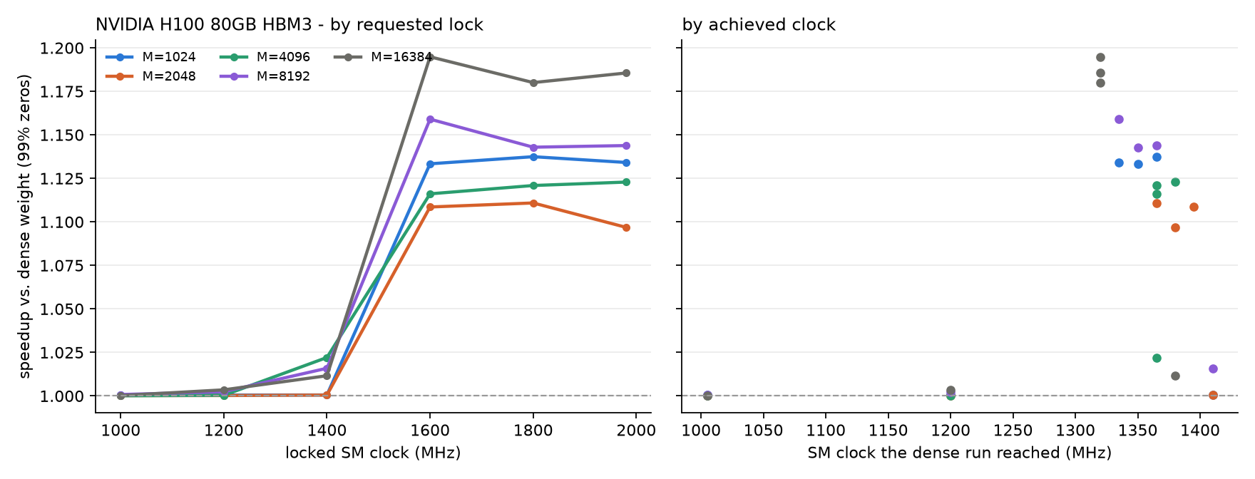
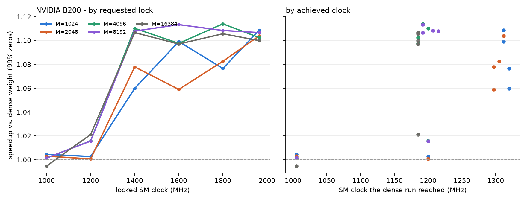
- Low locks: no effect. At 1000 and 1200 MHz the H100 is within 0.4% of dense for every
Mand every sparsity level, and the B200 is within 0.6% at 1000 MHz. The GPU holds the requested clock, so the work takes the same time whatever is in the weights. - High locks: the speedup comes back. On the H100 it is mixed at 1400 MHz (0.92-1.02x) and fully back, at its free-running size, from 1600 MHz up. On the B200 it is back from 1400 MHz, and partly there already at 1200 MHz (up to 1.02x for the larger shapes). Above that the lock stops being the binding constraint: dense runs reach only 1320-1410 MHz on the H100 and 1185-1320 MHz on the B200 no matter how high we set the lock, because the power limit decides the clock. Sparser weights draw less power, so they sustain a somewhat higher clock.
- How to read the right-hand panels. Each dot is one locked-clock setting for one
M(color isM, as on the left). Its height is the same 99%-zero speedup as on the left, but its horizontal position is the SM clock the dense run actually reached under that lock, not the lock itself. Dots for low locks sit at their locked clock; dots for locks the GPU cannot sustain slide left to wherever the power limit holds the clock. The clock is the median of 5 NVML samples, one per timing round, so it is a spot reading rather than an average and can be noisy. The 1600-1980 MHz locks all land on top of each other at about 1320-1400 MHz, which is why they give the same speedup. The 1400 MHz lock reaches a similar clock yet shows little speedup, so the sampled clock alone does not predict the effect; what matters is whether the power limit is binding. - It is a power effect, not a compute effect. The kernel does the same work. It only runs faster when the GPU is power-limited and the zeros let it hold a higher clock; at a clock the GPU can sustain, the time is identical.
Full results: every M and sparsity level, locked clocks
H100, 1000 MHz
| M | 5% | 10% | 25% | 50% | 70% | 90% | 99% |
|---|---|---|---|---|---|---|---|
| 1024 | 1.000 | 1.000 | 1.000 | 1.000 | 1.000 | 1.000 | 1.000 |
| 2048 | 1.000 | 1.000 | 1.000 | 1.000 | 1.000 | 1.000 | 1.000 |
| 4096 | 1.000 | 1.000 | 1.000 | 1.000 | 1.000 | 1.000 | 1.000 |
| 8192 | 1.000 | 1.000 | 1.000 | 1.000 | 1.001 | 1.001 | 1.001 |
| 16384 | 1.000 | 1.000 | 1.000 | 1.000 | 1.000 | 1.000 | 1.000 |
H100, 1200 MHz
| M | 5% | 10% | 25% | 50% | 70% | 90% | 99% |
|---|---|---|---|---|---|---|---|
| 1024 | 0.998 | 1.000 | 1.000 | 1.000 | 1.001 | 1.000 | 1.000 |
| 2048 | 1.000 | 0.997 | 1.000 | 1.000 | 1.000 | 1.000 | 1.000 |
| 4096 | 0.998 | 1.000 | 1.000 | 1.000 | 1.000 | 1.000 | 1.000 |
| 8192 | 1.000 | 1.002 | 1.000 | 1.002 | 1.002 | 1.003 | 1.002 |
| 16384 | 1.003 | 1.002 | 0.999 | 0.999 | 1.004 | 1.004 | 1.004 |
H100, 1400 MHz
| M | 5% | 10% | 25% | 50% | 70% | 90% | 99% |
|---|---|---|---|---|---|---|---|
| 1024 | 1.000 | 1.000 | 1.001 | 1.001 | 1.001 | 1.002 | 1.001 |
| 2048 | 1.000 | 1.000 | 1.001 | 1.001 | 1.001 | 1.001 | 1.000 |
| 4096 | 1.010 | 1.018 | 1.022 | 1.020 | 1.022 | 1.022 | 1.022 |
| 8192 | 1.008 | 1.013 | 1.014 | 1.014 | 1.016 | 1.015 | 1.016 |
| 16384 | 0.975 | 0.916 | 0.947 | 1.002 | 1.009 | 1.011 | 1.012 |
H100, 1600 MHz
| M | 5% | 10% | 25% | 50% | 70% | 90% | 99% |
|---|---|---|---|---|---|---|---|
| 1024 | 1.002 | 1.005 | 1.007 | 1.043 | 1.059 | 1.123 | 1.133 |
| 2048 | 0.988 | 0.978 | 0.988 | 1.004 | 1.028 | 1.096 | 1.109 |
| 4096 | 0.999 | 0.983 | 1.001 | 1.032 | 1.074 | 1.106 | 1.116 |
| 8192 | 1.026 | 1.022 | 1.026 | 1.046 | 1.093 | 1.128 | 1.159 |
| 16384 | 1.017 | 1.008 | 0.993 | 1.025 | 1.082 | 1.162 | 1.195 |
H100, 1800 MHz
| M | 5% | 10% | 25% | 50% | 70% | 90% | 99% |
|---|---|---|---|---|---|---|---|
| 1024 | 1.000 | 1.001 | 1.001 | 1.008 | 1.062 | 1.123 | 1.137 |
| 2048 | 0.992 | 0.992 | 0.984 | 1.016 | 1.042 | 1.100 | 1.111 |
| 4096 | 0.989 | 0.996 | 0.994 | 1.041 | 1.068 | 1.108 | 1.121 |
| 8192 | 1.021 | 1.017 | 1.021 | 1.044 | 1.077 | 1.120 | 1.143 |
| 16384 | 0.999 | 0.988 | 0.974 | 1.006 | 1.050 | 1.142 | 1.180 |
H100, 1980 MHz
| M | 5% | 10% | 25% | 50% | 70% | 90% | 99% |
|---|---|---|---|---|---|---|---|
| 1024 | 1.000 | 0.999 | 1.009 | 1.040 | 1.063 | 1.117 | 1.134 |
| 2048 | 0.990 | 0.990 | 0.990 | 1.000 | 1.047 | 1.093 | 1.097 |
| 4096 | 0.998 | 0.986 | 1.003 | 1.045 | 1.066 | 1.104 | 1.123 |
| 8192 | 1.013 | 1.020 | 1.015 | 1.046 | 1.064 | 1.122 | 1.144 |
| 16384 | 1.015 | 0.992 | 0.984 | 1.016 | 1.070 | 1.148 | 1.186 |
B200, 1000 MHz
| M | 5% | 10% | 25% | 50% | 70% | 90% | 99% |
|---|---|---|---|---|---|---|---|
| 1024 | 1.000 | 1.000 | 1.001 | 1.002 | 1.003 | 1.005 | 1.004 |
| 2048 | 1.001 | 1.000 | 1.001 | 1.001 | 1.002 | 1.003 | 1.003 |
| 4096 | 1.000 | 0.999 | 1.001 | 1.001 | 1.001 | 1.000 | 1.001 |
| 8192 | 1.000 | 1.000 | 1.001 | 1.001 | 1.002 | 1.002 | 1.001 |
| 16384 | 1.000 | 1.000 | 0.998 | 0.994 | 0.995 | 0.995 | 0.995 |
B200, 1200 MHz
| M | 5% | 10% | 25% | 50% | 70% | 90% | 99% |
|---|---|---|---|---|---|---|---|
| 1024 | 1.000 | 1.000 | 1.001 | 1.002 | 1.002 | 1.003 | 1.003 |
| 2048 | 1.000 | 1.000 | 1.000 | 1.001 | 1.001 | 1.001 | 1.001 |
| 4096 | 0.993 | 1.007 | 1.014 | 1.015 | 1.015 | 1.015 | 1.016 |
| 8192 | 0.989 | 0.992 | 1.015 | 1.015 | 1.016 | 1.016 | 1.016 |
| 16384 | 1.004 | 1.002 | 1.008 | 1.021 | 1.021 | 1.021 | 1.021 |
B200, 1400 MHz
| M | 5% | 10% | 25% | 50% | 70% | 90% | 99% |
|---|---|---|---|---|---|---|---|
| 1024 | 1.000 | 1.002 | 1.022 | 1.046 | 1.057 | 1.059 | 1.060 |
| 2048 | 1.006 | 0.996 | 1.002 | 1.027 | 1.059 | 1.065 | 1.078 |
| 4096 | 0.997 | 0.994 | 1.015 | 1.033 | 1.056 | 1.073 | 1.110 |
| 8192 | 0.987 | 1.005 | 1.011 | 1.034 | 1.060 | 1.079 | 1.108 |
| 16384 | 1.004 | 1.003 | 1.012 | 1.034 | 1.062 | 1.096 | 1.107 |
B200, 1600 MHz
| M | 5% | 10% | 25% | 50% | 70% | 90% | 99% |
|---|---|---|---|---|---|---|---|
| 1024 | 1.001 | 1.002 | 1.029 | 1.046 | 1.070 | 1.073 | 1.099 |
| 2048 | 1.001 | 1.003 | 1.013 | 1.030 | 1.045 | 1.058 | 1.059 |
| 4096 | 0.996 | 0.987 | 0.997 | 1.031 | 1.049 | 1.071 | 1.098 |
| 8192 | 1.009 | 0.996 | 1.026 | 1.043 | 1.072 | 1.105 | 1.113 |
| 16384 | 1.001 | 1.001 | 1.006 | 1.034 | 1.058 | 1.093 | 1.097 |
B200, 1800 MHz
| M | 5% | 10% | 25% | 50% | 70% | 90% | 99% |
|---|---|---|---|---|---|---|---|
| 1024 | 1.001 | 1.002 | 1.015 | 1.043 | 1.078 | 1.037 | 1.077 |
| 2048 | 0.987 | 0.986 | 0.990 | 1.009 | 1.041 | 1.052 | 1.083 |
| 4096 | 0.994 | 1.000 | 1.004 | 1.042 | 1.057 | 1.074 | 1.114 |
| 8192 | 0.987 | 1.003 | 1.017 | 1.038 | 1.059 | 1.095 | 1.108 |
| 16384 | 1.003 | 1.003 | 1.011 | 1.034 | 1.061 | 1.095 | 1.106 |
B200, 1965 MHz
| M | 5% | 10% | 25% | 50% | 70% | 90% | 99% |
|---|---|---|---|---|---|---|---|
| 1024 | 1.000 | 0.996 | 1.005 | 1.043 | 1.067 | 1.054 | 1.109 |
| 2048 | 1.009 | 1.000 | 1.017 | 1.029 | 1.050 | 1.074 | 1.104 |
| 4096 | 1.000 | 0.993 | 1.009 | 1.034 | 1.054 | 1.074 | 1.102 |
| 8192 | 0.997 | 1.011 | 1.011 | 1.032 | 1.057 | 1.093 | 1.107 |
| 16384 | 1.000 | 0.999 | 1.004 | 1.029 | 1.059 | 1.090 | 1.100 |
What this means for LLM inference
The two experiments give two conditions for a speedup:
- The matmul has to be big enough to be compute-bound. Only then is the matmul’s speed set by the clock, and only then does the GPU sit at its power cap and throttle. A small matmul is limited by how fast the weights can be read from memory, so even a higher clock would not make it finish sooner.
- The input has to be very sparse. The gains need 50% or more zeros, and are only large at 90-99%.
The first condition comes down to M, the number of tokens multiplied by the weight at once. An M x K by K x N bf16 matmul does 2MKN FLOPs and reads roughly 2KN bytes of weights, so it does about M FLOPs per byte. The H100 and B200 can do roughly 300 bf16 FLOPs per byte of memory bandwidth, so below a few hundred tokens a matmul is memory-bound and above that it is compute-bound. In inference that maps directly onto the two phases:
- Prefill processes the whole prompt at once, so
Mis thousands of tokens and the matmuls are compute-bound. - Decode generates one token per sequence per step, so
Mis the batch size, typically tens to low hundreds, and the matmuls are memory-bound. Mixture-of-experts layers make this even smaller: each expert only sees the tokens routed to it.
Our results line up with this split. In the exploratory H100 run with 1, 16 and 128 rows, zeros made no difference (within 0.5%), while from 1024 rows up the speedup at 99% zeros was 1.08-1.18x across both GPUs, and the clock locks showed it comes from the power-limited clock.
Limitations: bf16 only, random Gaussian weights rather than trained ones, a single square weight shape, one GPU of each type, and power readings from NVML are sampled, not integrated. Natural follow-ups are to repeat this with the weight shapes of a real model, to compare against a genuine semi-structured sparse kernel path such as cuSPARSELt, and to run the same tests in fp8.