By Pramodith B, Member of Technical Staff
Are you using the right baseline for your kernel benchmarks? An analysis of torch.compile modes
One of the first things that a Kernel Engineer does when they’re tasked with creating an optimized kernel is, establishing a fair baseline. It’s common to initially implement or import a PyTorch kernel and establish it as the reference point for both accuracy and performance. However, running a PyTorch kernel in eager mode is very inefficient since every line of code is executed one at a time, and the Python interpreter has to manage the execution of each operation. Moreover, the lack of operator/kernel fusion forces the program to write intermediate results to global memory between every operation. This can lead to significant overhead and suboptimal performance, especially for complex computations.
torch.compile addresses these issues by compiling the Python code into optimized Triton kernels (GPU) or C++ (CPU), creating graphs that can optimize the whole kernel by removing redundant operations, fusing operators together, and optimizing memory access patterns. This results in significantly improved performance compared to eager mode.
Using torch.compile is as simple as wrapping your PyTorch kernel with torch.compile and running it. The ease of adoption coupled with the significant performance improvements that compilation provides makes it an attractive and realistic baseline for benchmarking optimized kernels against.
torch.compile modes
torch.compile provides 4 different modes of compilation, each with its own trade-offs between compilation time and runtime performance. Per the PyTorch documentation, the modes are:
defaultis the default mode, which is a good balance between performance and overhead
reduce-overheadis a mode that reduces the overhead of python with CUDA graphs, useful for small batches. Reduction of overhead can come at the cost of more memory usage, as we will cache the workspace memory required for the invocation so that we do not have to reallocate it on subsequent runs. Reduction of overhead is not guaranteed to work; today, we only reduce overhead for CUDA only graphs which do not mutate inputs. There are other circumstances where CUDA graphs are not applicable; use TORCH_LOGS=perf_hints to debug.
max-autotuneis a mode that leverages Triton or template based matrix multiplications on supported devices and Triton based convolutions on GPU. It enables CUDA graphs by default on GPU.
max-autotune-no-cudagraphsis a mode similar tomax-autotunebut without CUDA graphs
Switching compilation modes is as simple as passing the mode argument to torch.compile:
compiled_fn = torch.compile(fn, mode="max-autotune")
This raises the question - which torch.compile mode should you use as a baseline?
When you take a look at popular open source kernel repositories the most commonly used baselines are:
- eager execution
torch.compilewithdefaultmodetorch.compilewithmax-autotunemode
max-autotune doesn’t guarantee the best speedup
In the past few months that we’ve spent implementing kernels, we noticed that max-autotune often didn’t produce the best performing (speed) compiled kernel, and in some cases, even running the kernel in eager mode produced better performing kernels than max-autotune. In fact, we believe that while there is no one-size-fits-all answer to which torch.compile mode is best for benchmarking, both max-autotune-no-cudagraphs and default stand head-and-shoulders above the rest and can often be the best choice.
Experimental Setup
In order to validate max-autotune-no-cudagraphs as the best mode for benchmarking, we ran a comprehensive study comparing the performance of the different torch.compile modes across a wide variety of kernels. The kernels were sourced from commonly used operations/modules in building LLMs/VLMs and included a mix of GEMM-heavy, memory-bound, and reduction-heavy kernels. We ran each workload in eager, default, reduce-overhead, max-autotune, and max-autotune-no-cudagraphs modes, and measured the latency of each.
Each kernel, mode pair for a given shape is profiled in a new sub-process to ensure that CUDA contexts and torch.compile caches never bleed between runs.
A comprehensive list of the workloads and what they represent is provided in the appendix. The code for reproducing the experiment can be found here.
Profiling
In order to get accurate latency measurements, we used the Triton do_bench profiler which runs the kernel multiple times and reports the median latency.
In order to ensure that we only profile the kernel execution time and not the compilation time, we run the kernel through a warmup loop of 20 iterations immediately after it is compiled. Additionally, we set the the warmup and rep parameters of do_bench to 100 (ms) and 1000 (ms) respectively, to ensure that we get stable latency measurements.
The warmup and rep parameters in the do_bench profiler are in milliseconds, and internally they are used to determine how many warmup iterations and actual profiling iterations a kernel goes through so setting these appropriately is important to get accurate latency measurements. If the latency of a kernel is 1000 (ms) i.e. 1 second and you set rep to 100, the profiler will only run the kernel one time leading to timing measurements that aren’t robust. With rep=1000, even our slowest workload (llm_kl_divergence_loss prefill at ~13ms) gets ~78 profiling iterations, while the median workload gets ~20,000. This ensures all reported medians are well-sampled.
In order to ensure that we capture shapes seen during both training/prefill and inference/decoding we ran each workload with two different shape presets - one representing typical shapes seen during decoding and one representing typical shapes seen during prefill.
The full shape configuration for each preset can be found in the appendix too.
All 23 workloads are profiled on the prefill shape preset. For the decode preset we exclude 5 workloads whose input shapes are invariant to the preset (vlm_contrastive_nce_loss, diff_vae_decoder_upsample, diff_time_embedding_mlp, rl_dpo_loss, rl_grpo_loss since these are either training-only losses or operations with architecture-fixed spatial dimensions), leaving 18 decode workloads. Each workload instance is profiled across all compilation modes plus eager, giving a total of 41 workload instances (shape x workload).
Results
All the workloads were profiled on a H100 80GB HBM3 device. We used PyTorch 2.9.1 and CUDA 13. For quantifying the modes we use the following metrics:
- Wins: For each workload, we determine which mode had the lowest latency and count that as a “win” for the mode. This gives us a simple count of how many workloads each mode performed best on.
- Geometric mean speedup vs eager: For each workload, we calculate the speedup of each mode compared to
eagermode by dividing the latency of theeagermode by the latency of the mode in question. We then take the geometric mean of these speedups across all workloads to get an overall sense of how much faster each mode is compared toeager. - Average win margin %: For the two strongest modes (
defaultandmax-autotune-no-cudagraphs), we compute how much faster the winner is compared to the loser as a percentage of the loser’s latency, averaged across the workloads each mode wins. This tells us not just how often a mode wins, but by how much.
The raw results for each workload and mode can be found here.
Prefill workloads
Out of 23 prefill workloads, max-autotune-no-cudagraphs wins 17, default wins 4, max-autotune wins 1, and eager wins 1. reduce-overhead wins none.
| Mode | Wins | Winning workloads |
|---|---|---|
max-autotune-no-cudagraphs |
17 | diff_cfg_blend, diff_time_embedding_mlp, diff_unet_resblock, diff_vae_decoder_upsample, llm_gelu_mlp, llm_kl_divergence_loss, llm_label_smoothed_ce_loss, llm_layernorm, llm_logits_projection_softmax, llm_moe_router, llm_qk_norm, llm_rmsnorm, llm_swiglu_mlp, rl_ppo_clipped_loss, vlm_patch_embedding_conv2d, vlm_vision_rmsnorm_pool, vlm_vit_mlp_block |
default |
4 | diff_scheduler_step, llm_rope_apply, rl_dpo_loss, rl_grpo_loss |
max-autotune |
1 | vlm_contrastive_nce_loss |
eager |
1 | llm_topk_sampling_prep |
reduce-overhead |
0 | — |
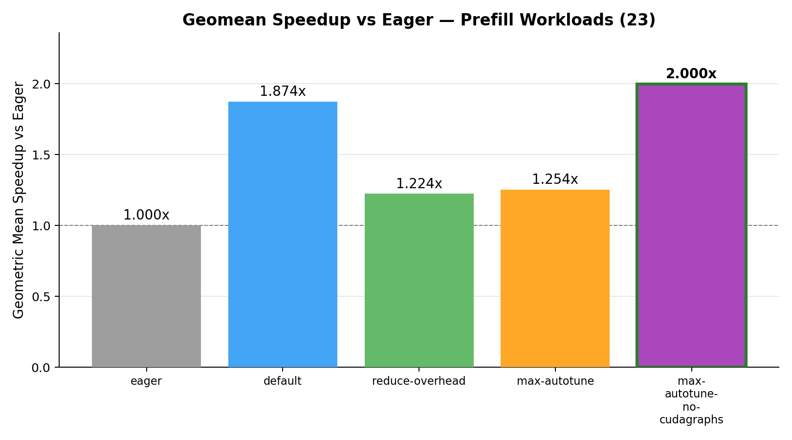
Geometric mean speedup vs eager:
We can see that all the torch.compile modes provide significant speedups over eager mode, but default and max-autotune-no-cudagraphs provide the best geomean speedups nearly twice as fast as eager, with max-autotune-no-cudagraphs being the best overall.
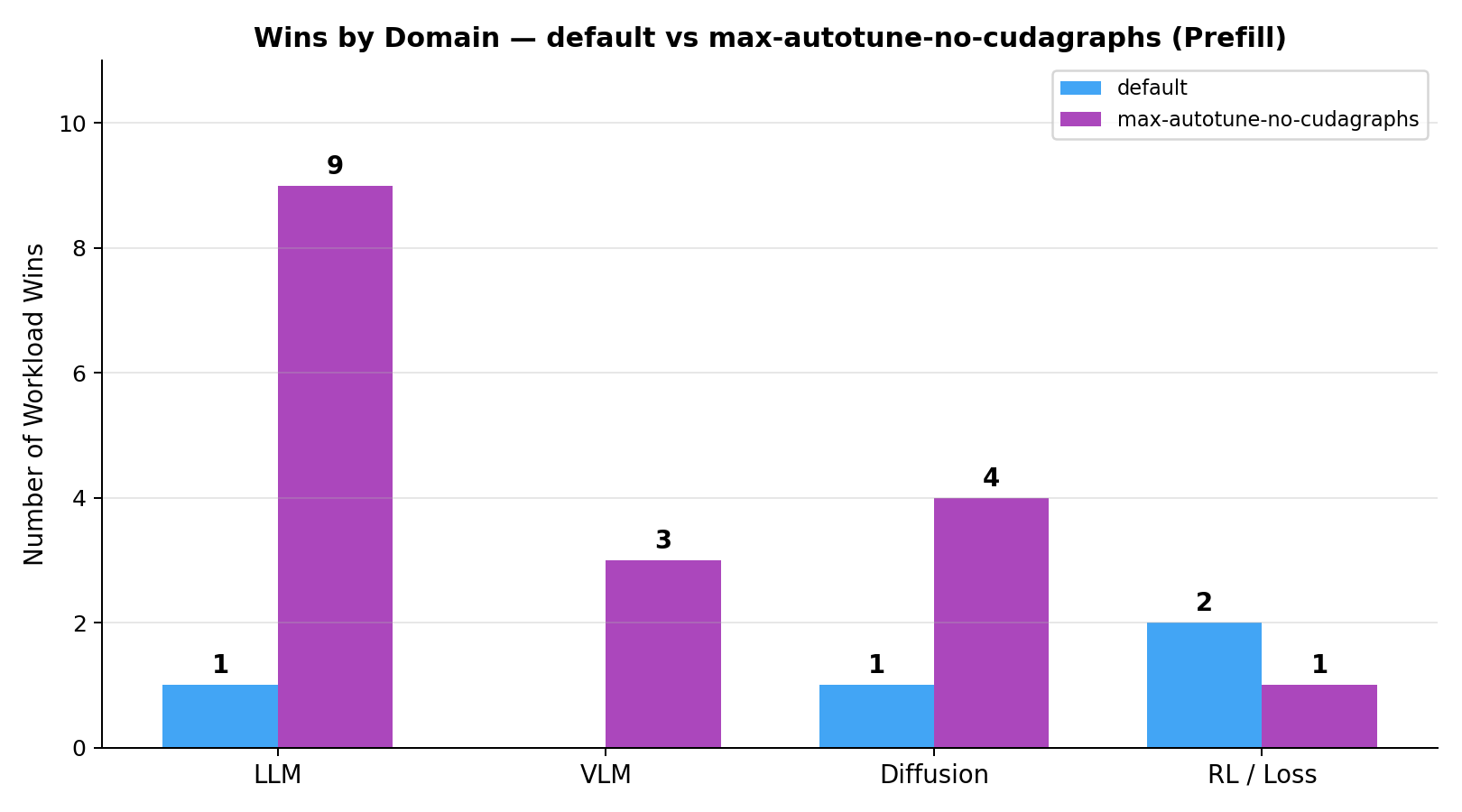
Breaking down wins by domain (type of kernel) for the two strongest modes (default vs max-autotune-no-cudagraphs):
 Average win margin (
default vs max-autotune-no-cudagraphs):
We can observe that max-autotune-no-cudagraphs not only wins more workloads than default, but also has a higher average win margin, meaning that when it wins, it tends to outperform default by a larger percentage compared to how much default outperforms it when it wins.
| Mode | Wins | Avg win margin |
|---|---|---|
max-autotune-no-cudagraphs |
17 | 7.58% |
default |
4 | 2.45% |
Decode workloads
On the decode workloads we observe that default has the most wins but the gap between default and max-autotune-no-cudagraphs is much narrower compared to the prefill workloads. Out of 18 decode workloads, default wins 10 and max-autotune-no-cudagraphs wins 8. Neither max-autotune, reduce-overhead, nor eager wins any.
| Mode | Wins | Winning workloads |
|---|---|---|
default |
10 | diff_cfg_blend, diff_scheduler_step, diff_unet_resblock, llm_gelu_mlp, llm_kl_divergence_loss, llm_layernorm, llm_moe_router, llm_rope_apply, llm_topk_sampling_prep, rl_ppo_clipped_loss |
max-autotune-no-cudagraphs |
8 | llm_label_smoothed_ce_loss, llm_logits_projection_softmax, llm_qk_norm, llm_rmsnorm, llm_swiglu_mlp, vlm_patch_embedding_conv2d, vlm_vision_rmsnorm_pool, vlm_vit_mlp_block |
max-autotune |
0 | — |
reduce-overhead |
0 | — |
eager |
0 | — |
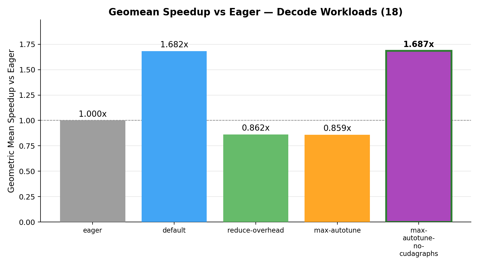
Geometric mean speedup vs eager:
For decode workloads reduce-overhead and max-autotune actually perform worse than eager (below 1.0x), while default and max-autotune-no-cudagraphs provide significant speedups and are virtually tied.
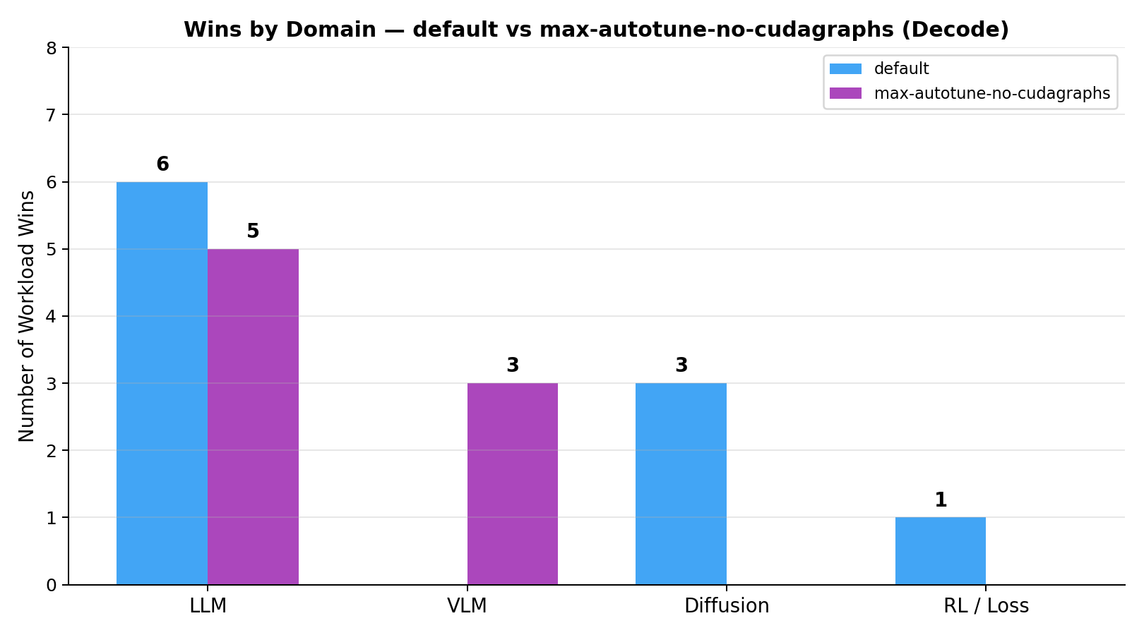
Breaking down wins by domain for the two strongest modes:
 Average win margin (
default vs max-autotune-no-cudagraphs):
The win margins being very similar for the two dominant modes re-iterates how closely matched the two modes are on the decode workloads.
| Mode | Wins | Avg win margin |
|---|---|---|
default |
10 | 5.94% |
max-autotune-no-cudagraphs |
8 | 6.83% |
Why cudagraphs might be hurting performance
Both max-autotune and reduce-overhead enable CUDA graphs, in fact the only difference between max-autotune and max-autotune-no-cudagraphs is the presence of CUDA graphs.
CUDA graphs are great for reducing the overhead involved with launching multiple CUDA kernels, which is what you’d have with an end-to-end model running a forward/backward pass.
However, in an isolated single-kernel benchmark there is no multi-kernel launch sequence to optimize away. Instead, CUDA graph replay introduces a fixed latency floor (~0.02ms in our measurements) that is more expensive than a regular single-kernel launch.
Issues with the performance of max-autotune have also been observed by others. Horace He mentions how it introduces extra memcpy on entry and exit. Ian Barber’s blog mentions that in one instance it introduces an extra fusion that slowed down the kernel. It’s likely that the performance impact of CUDA graphs is workload-dependent, which is why we see it hurting performance on some workloads but not others. There’s also an unresolved issue on Pytorch regarding the underperformance of max-autotune and reduce-overhead.
Conclusion
Using torch.compile is the easiest way to create an optimized version of an eager kernel. If you’re a kernel engineer your challenge is to out-perform torch.compile’s optimizations with your own hand-crafted kernel, so it only makes sense to use the best optimized torch.compile mode as your baseline.
Unfortunately, there isn’t a single torch.compile mode that yields the best performance. Despite the moniker max-autotune, it doesn’t always produce the best performing compiled kernel, and in some cases, even running the kernel in eager mode produces better performing kernels than max-autotune.
Consequently it’s important to evaluate the different torch.compile modes and choose the best performing one as your baseline. Based on our experiments, we found that max-autotune-no-cudagraphs is the best performing mode for prefill/training workloads. For decode workloads, default but the two modes are effectively tied on geomean speedup (1.687x vs 1.682x).
Appendix
Workload Descriptions
| Workload Name | Description |
|---|---|
llm_rmsnorm |
Root Mean Square Layer Normalization used in Llama, Qwen, Mistral, and most modern LLMs. Normalises by RMS instead of mean+variance, omitting the bias term. |
llm_layernorm |
Standard Layer Normalization with learnable affine parameters. Used in BERT-style encoders, GPT-2, and ViT models. |
llm_swiglu_mlp |
SwiGLU MLP block: silu(x @ Wg) * (x @ Wu) @ Wd. Fused gate-and-up projection is the dominant cost. Used in Llama, Mistral, Qwen, and DeepSeek. |
llm_gelu_mlp |
Two-layer MLP with tanh-approximate GELU activation: gelu(x @ W1) @ W2. Used in GPT-2, BERT, and ViT models. |
llm_rope_apply |
Rotary Position Embeddings (RoPE) applied to query/key tensors by rotating even/odd dimension pairs using pre-computed cos/sin tables. |
llm_logits_projection_softmax |
Language-model head GEMM over the full vocabulary (32768) followed by softmax, representing the peak memory-bandwidth and compute cost per forward pass. |
llm_topk_sampling_prep |
Top-k sampling pipeline: softmax over vocabulary logits, retain top-32 candidates, renormalise, and select. Models the token-sampling pipeline during autoregressive decode. |
llm_moe_router |
Mixture-of-Experts router: linear projection to 64 expert logits, softmax, and top-2 dispatch. Used in Mixtral, DeepSeek-MoE, and Qwen-MoE. |
llm_qk_norm |
L2-normalise query and key tensors along the head dimension (QK-Norm). Stabilises attention logit magnitudes for long contexts. Used in Gemma 2 and Chameleon. |
vlm_patch_embedding_conv2d |
ViT patch embedding: stride-14 conv2d followed by spatial flatten and transpose. Used in CLIP, SigLIP, InternViT, and similar vision encoders. |
vlm_vit_mlp_block |
ViT MLP block: pre-LayerNorm, GELU MLP, and residual addition. One complete FFN sub-block of a Vision Transformer encoder layer. |
vlm_vision_rmsnorm_pool |
RMSNorm followed by mean pooling over the sequence dimension. Produces a fixed-size vision embedding from patch tokens for VLM visual projectors. |
vlm_contrastive_nce_loss |
Symmetric InfoNCE (CLIP-style) contrastive loss. L2-normalises image and text embeddings and computes bidirectional cross-entropy. Used in CLIP, SigLIP, and ALIGN. |
diff_unet_resblock |
U-Net residual block: GroupNorm, SiLU, two Conv3x3 layers, and skip-connection add. Standard ResNet-style block used in Stable Diffusion’s U-Net backbone. |
diff_vae_decoder_upsample |
VAE decoder upsample block: nearest-neighbour 2x interpolation, SiLU, and two Conv3x3 layers. Used in Stable Diffusion and SDXL decoder paths. |
diff_time_embedding_mlp |
Sinusoidal timestep embedding MLP: converts scalar diffusion timesteps into a high-dimensional conditioning vector via sinusoidal encoding and a two-layer SiLU MLP. Used in DDPM and DiT. |
diff_cfg_blend |
Classifier-Free Guidance linear blend: uncond + scale * (cond - uncond). Pure elementwise operation on full latent tensors, memory-bandwidth bound. |
diff_scheduler_step |
Single DDPM/DDIM scheduler denoising step: latents - sigma * noise with per-batch sigma broadcast. One step of the iterative reverse-diffusion process. |
llm_label_smoothed_ce_loss |
Label-smoothed cross-entropy loss over a 32768-token vocabulary. Mixes hard-target NLL with uniform smoothing to prevent overconfident predictions. |
llm_kl_divergence_loss |
Temperature-scaled KL divergence for knowledge distillation. Used in DistilBERT, MiniLM, and RLHF reward-model distillation. |
rl_ppo_clipped_loss |
PPO clipped surrogate policy-gradient objective. Prevents large policy updates by clipping the probability ratio. Used in InstructGPT and RLHF fine-tuning. |
rl_dpo_loss |
Direct Preference Optimization loss. Optimises a language model to prefer chosen completions over rejected ones without a separate reward model. Used in Zephyr and OpenHermes. |
rl_grpo_loss |
Group Relative Policy Optimization loss. Eliminates the critic by normalising rewards within a group of 8 completions per prompt. Used in DeepSeekMath and DeepSeek-R1. |
Shape Presets
| Parameter | Decode | Prefill |
|---|---|---|
Batch size (b) |
64 | 16 |
Sequence length (s) |
1 | 2048 |
Hidden dimension (h) |
2048 | 2048 |
| Attention heads | 16 | 16 |
Head dimension (d) |
128 | 128 |
| Intermediate size (MLP) | 5504 | 5504 |
| Vocabulary size | 32768 | 32768 |
| VLM image size | 224x224 | 448x448 |
| VLM patch tokens | 196 | 1024 |
| VLM embed dimension | 1024 | 1024 |
| Diffusion U-Net feature map | 32x32 | 64x64 |
| Diffusion latent map | 64x64 | 128x128 |
| U-Net channels | 320 | 320 |
| VAE decoder channels | 256 | 256 |
| Contrastive loss pairs | 256 | 256 |
| RL loss samples (DPO, GRPO) | 512 | 512 |