By Jack Foxabbott, Founding Member of Technical Staff
Diversity Is All You Need (To Converge): Why Evolutionary Algorithms Need Diversity Management
Evolutionary algorithms are simple: maintain a population, evaluate fitness, keep the best, mutate to create offspring, and repeat. But they routinely fail in practice, and the reason is almost always the same: the population’s diversity wasn’t managed properly.
Selection wants to collapse the population into a monoculture. Mutation wants to smear it back out. If you don’t manage that tension you either collapse into a local optimum and sit there, or keep “exploring” forever and never cash it in. Getting it right is the difference between polynomial and exponential runtime.
We’ll build intuition on a multimodal landscape (Rastrigin), then anchor that intuition in five theoretical results about convergence speed and how it depends on the exploration/exploitation balance. These results are mostly proved on stylised toy landscapes (bit strings, synthetic traps), because that’s where the maths is sharp enough to separate polynomial-time from exponential-time behaviour. The proofs pin down exactly when “keep the best and mutate” is fast, slow, or outright doomed. The toy settings are deliberately simple, but the failure modes they expose (premature convergence from too much selection, random-walk behaviour from too much mutation) are the same ones that show up on real problems.
The Rastrigin function
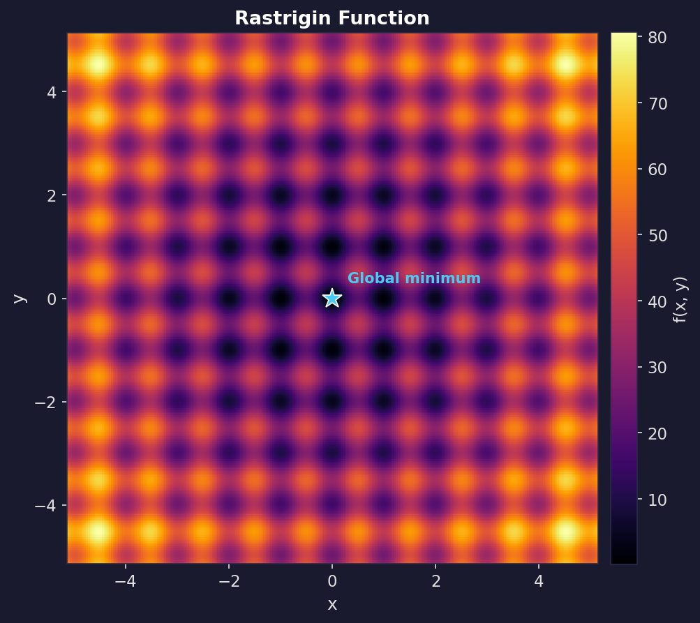
The Rastrigin function is a standard optimisation test problem because it’s regularly packed with local minima: it looks like a rippled bowl, where the global best point is the bottom of the bowl, but there are many local dents along the way.
In two dimensions:
\[f(x, y) = 20 + (x^2 - 10\cos(2\pi x)) + (y^2 - 10\cos(2\pi y)).\]The global minimum is at $(0,0)$ with $f(0,0) = 0$. Any greedy, hill-climbing algorithm gets stuck, which makes it a good test of whether an optimiser actually explores.
The EA
We ran the same EA on the Rastrigin function three times, varying two knobs: selection pressure and mutation strength. Everything else was identical: population size 30, elitism (always keep the best individual found so far), Gaussian mutation. The only thing changing is how quickly selection collapses diversity, versus how quickly mutation replenishes it.
Selection here uses tournament selection: to choose each parent, pick $k$ individuals at random from the population and keep the fittest. Larger $k$ means stronger pressure toward the current best. Mutation uses Gaussian perturbation: add a random offset drawn from $\mathcal{N}(0, \sigma^2)$ to each coordinate of the parent. Larger $\sigma$ means bigger jumps, so more exploration but also more disruption of good solutions.
Many EAs also use crossover (also called recombination): pick two parents and combine parts of each to produce a child. For bit strings this might mean taking the first half of one parent and the second half of the other; for continuous vectors it might mean averaging or blending coordinates. Crossover is different from mutation because it doesn’t introduce new information, it rearranges what’s already in the population. Our Rastrigin demo doesn’t use crossover, but it plays a central role in the theoretical results below.
Too little diversity
Tournament selection with size 10 (very aggressive, almost always picks the single best individual). Gaussian mutations with $\sigma = 0.15$.
The population collapses in a handful of generations. You get “fast convergence”… to the wrong thing. The mutation steps are too small to hop the ridges between basins. What looks like decisive progress is selection doing what it always does: removing variety.
Too much diversity
Tournament selection with size 2 (almost random). Gaussian mutations with $\sigma = 3.5$.
This is the opposite failure mode: diversity is maximal, but unstructured, and each generation is basically a fresh random sample. Selection isn’t strong enough to amplify improvements into a stable lineage, so the algorithm can’t compound its gains.
Balanced diversity
Tournament selection with size 5. Adaptive Gaussian mutations that start large and decay: $\sigma(t) = 1.2 \cdot (1 - 0.8\, t/T)$.
Early on, large mutations spread the population across the landscape, and as the algorithm progresses they shrink, focusing the population on the best basin until the global optimum is found.
Selection exploits by copying what works, while mutation explores by trying something new. The balanced case transitions from broad exploration to focused exploitation, while the other two cases get stuck at one extreme.
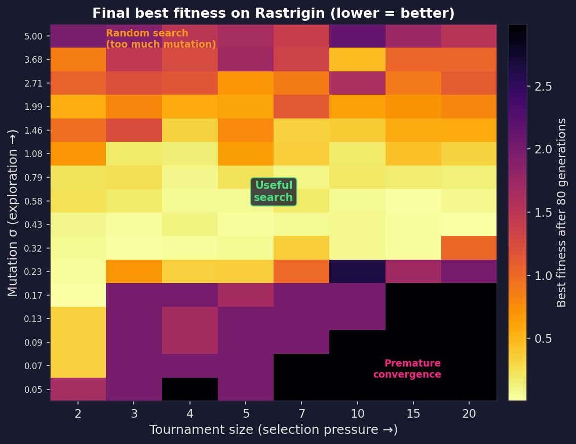
The full picture
These three runs are points in a larger space. The plot below sweeps across selection pressure (tournament size) and mutation strength ($\sigma$), running the same EA for each combination and recording the best fitness found. Bright cells reached the global optimum; dark cells got stuck. There’s a narrow diagonal of good settings; too aggressive on either axis and the algorithm fails in opposite ways.
Seeing it in the numbers
The time-series below plot best fitness and population diversity (average pairwise distance) over generations for all three regimes.
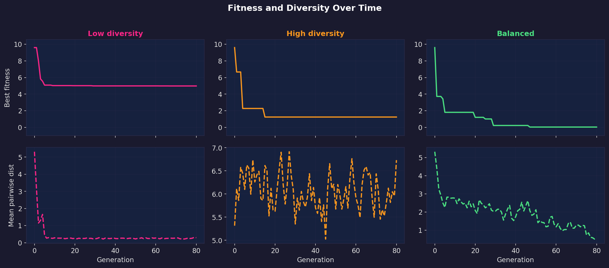
In the low-diversity run, diversity crashes immediately and fitness flatlines at a local optimum. In the high-diversity run, diversity stays high but fitness never improves because there’s no exploitation. In the balanced run, diversity starts high and decays smoothly while fitness steadily drops toward zero. That smooth handoff from exploration to exploitation is what makes the balanced run work.
Exploration and exploitation are two clocks
There are many ways to talk about “exploration vs exploitation”. The theory literature boils it down to two time scales, two clocks your EA is running at all times.
Clock 1: Takeover. How quickly selection fills the population with copies of the current best type, even if you turn mutation off. This is exploitation speed. It’s also a quantitative description of how quickly diversity disappears.
Clock 2: Escape. How quickly variation operators can produce something genuinely different (a new basin, a new building block, a gap-crossing move) despite selection trying to prune it away. On some landscapes, escape requires a rare event (flipping $k$ specific bits at once, or jumping a specific ridge), so the escape clock can easily become exponential if the population has collapsed.
A good diversity strategy doesn’t maximise diversity. It makes sure the escape clock beats the takeover clock early, then lets takeover win later.
Five theoretical results about convergence speed
The Rastrigin experiments and the two-clocks framing give intuition, but they don’t tell us why one setting works and another doesn’t, or how to predict what will happen on a new problem. For that we need theory.
The results below come from a branch of research called runtime analysis, which studies evolutionary algorithms the way complexity theory studies classical algorithms: by proving bounds on how many fitness evaluations an EA needs to find the optimum, as a function of problem size. The key question is whether that number is polynomial (feasible, scales reasonably) or superpolynomial/exponential (infeasible, blows up). Most of these results are proved for EAs operating on bit strings, because that’s a setting where the maths is tractable enough to get clean answers.
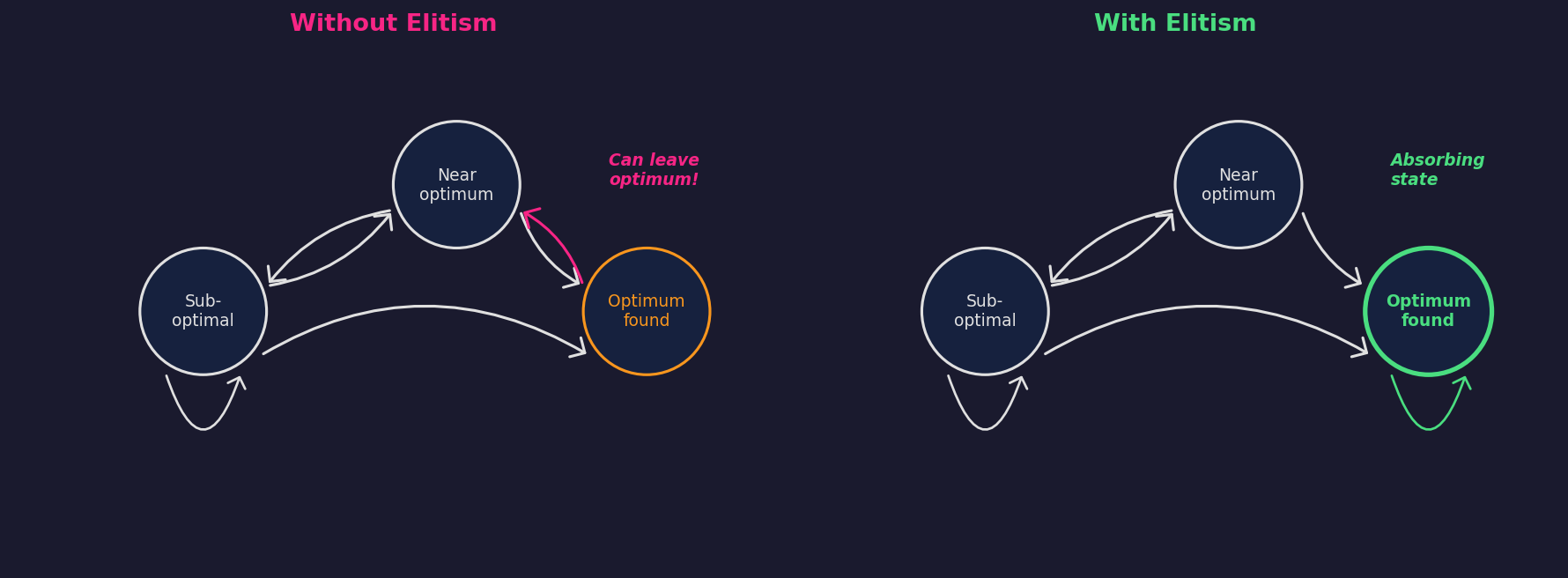
1. Elitism gives convergence, but not speed
The most fundamental question is: does the algorithm even converge to the global optimum? Rudolph (1994) used Markov chain analysis to prove two things about canonical genetic algorithms.
First, a negative result: without elitism, the standard GA never converges to the global optimum, regardless of initialisation, crossover operator, or objective function. The population’s state space is ergodic: it visits optimal states infinitely often but leaves them infinitely often. There are no absorbing states.
Second, a positive result: adding elitism (always preserving the best solution found so far) makes the set of populations containing a global optimum into an absorbing set. Combined with ergodicity of the mutation operator (any solution is reachable from any starting point with nonzero probability), the algorithm converges to the global optimum almost surely.
The conditions are mild (elitism is a one-line code change, and Gaussian mutation is ergodic by construction), but the theorem says nothing about how long convergence takes, and it could easily be exponential. That’s exactly what the Rastrigin GIFs demonstrate: elitism is on in all three runs, but only the balanced one is fast in any practical sense.
2. Selection pressure has a closed-form “diversity half-life”
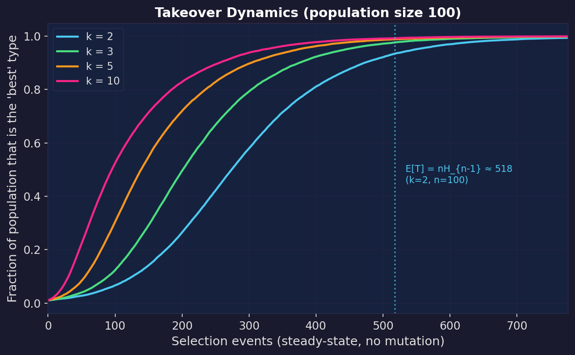
Selection pressure can be made precise, and the classic measure is takeover time: the expected number of selection iterations needed until the population consists entirely of copies of the initially-best individual (assuming it can’t go extinct).
Rudolph (2000) proved closed-form expressions for tournament selection with population size $n$. Recall that a tournament of size $k$ picks $k$ individuals at random and keeps the fittest; a binary tournament has $k = 2$, a ternary tournament has $k = 3$. In the “non-generational” variant, one individual is replaced at a time rather than rebuilding the whole population each generation. Under this scheme:
- Binary tournament ($k = 2$): $E[T] = n H_{n-1}$
- Ternary tournament ($k = 3$): $E[T] = \tfrac{2}{3}\, n H_{n-1}$
where $H_{n-1}$ is the $(n-1)$-th harmonic number ($H_{n-1} \approx \log n$).
Stronger tournaments shrink takeover time by a constant factor. You get faster exploitation, and also faster loss of diversity.
Once takeover happens, crossover starts recombining near-clones and mutation becomes the only source of novelty. At that point you’re effectively running a hillclimber with a particular step size distribution, often exactly the “too little diversity” regime from the Rastrigin experiments.
3. Mutation rate has a phase transition
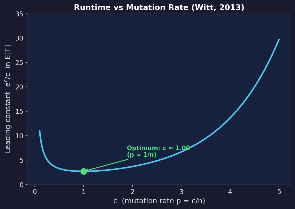
In standard bitwise mutation, each bit in the solution string is flipped independently with probability $p$. Witt (2013) proved tight bounds for the $(1+1)$ EA (the simplest elitist EA: keep one solution, produce one mutant, keep whichever is better) on any linear function over bit strings of length $n$.
If you set $p = c/n$ so that you flip $c$ bits per step on average, the expected runtime is $\approx \frac{e^c}{c} n \ln n$. This is minimised at $c = 1$ (i.e. $p = 1/n$, flipping about one bit per step), where it evaluates to $\approx e \cdot n \ln n$. The leading constant $e^c/c$ grows rapidly as you increase $c$: at $c = 3$ it’s already $\approx 6.7$ compared to $\approx 2.7$ at the optimum.
The result above holds when $c$ is a fixed number. But you can also ask: what if I let $c$ grow with problem size, flipping more bits on larger problems? Witt showed that as long as the expected number of flipped bits stays below $O(\ln n)$, the runtime is still polynomial in $n$. Beyond that, it becomes superpolynomial, meaning it grows faster than $n^k$ for any fixed $k$.
(A note on what “polynomial in $n$” means here: these results study how runtime scales across problems of different sizes. For any single problem, $n$ is fixed and the runtime is just a number. The value of the scaling analysis is that it tells you which strategies will remain feasible as problems get bigger, and which ones will hit a wall.)
This is the discrete analogue of the Rastrigin knobs. If you flip too many bits per step, you destroy good solutions faster than selection can exploit them. If you flip too few, you can’t escape local optima. The optimum is in between, and the $e^c/c$ curve quantifies the cost of getting it wrong.
4. Diversity plus crossover can change the exponent
Local optima are where diversity management has the sharpest effect on runtime.
A clean example is the $\text{Jump}_k$ function, a synthetic benchmark designed to test exactly this. It rewards solutions for having more 1-bits, except for a “gap” of width $k$ just below the optimum (the all-ones string). Solutions in the gap have artificially bad fitness, so the EA gets stuck on the edge of the gap, $k$ bits away from the optimum. The only way for a mutation-only algorithm to cross it is to flip the right $k$ bits in a single step.
Dang, Friedrich, Kötzing, Krejca, Lehre, Oliveto, Sudholt, and Sutton (2016) proved that a mutation-only $(1+1)$ EA needs $\Theta(n^k)$ fitness evaluations. But a population-based GA with crossover and diversity mechanisms solves the same problem in $O(n \log n)$, which is a completely different scaling law.
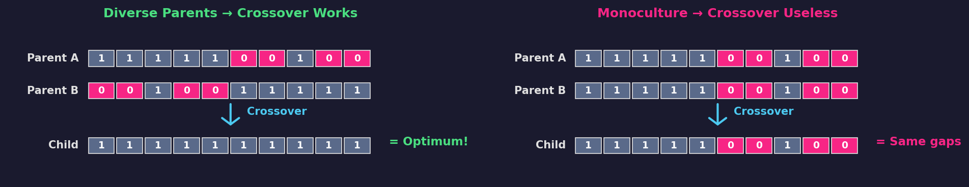
Why does diversity matter here? Because crossover is only powerful when it recombines different parents. Diversity mechanisms keep multiple distinct individuals alive on the plateau, so crossover can assemble the global optimum from complementary partial structures instead of waiting for a single lucky $k$-bit mutation. If selection collapses the population so that the plateau contains only near-identical individuals, crossover degenerates into “copy the same thing twice”, and you’re back to waiting $\Theta(n^k)$.
The journal version (Dang et al., 2018) studies seven diversity mechanisms and shows that all of them enable the exponential-to-polynomial speedup.
For a comprehensive survey of these results, see Sudholt (2018).
5. Self-adjustment can be provably optimal parameter control
The Rastrigin “balanced” run used a hand-designed decay schedule for $\sigma(t)$, but there’s theory saying you can do better: let the algorithm learn its mutation strength online.
Try a slightly bigger step and a slightly smaller step, then keep whichever produced the best offspring. Exploration and exploitation applied to the parameter choice itself, not just the search point.
Doerr, Gießen, Witt, and Yang (2019) proved that a $(1+\lambda)$ EA with this self-adjusting mutation rate finds the optimum on OneMax (the simplest benchmark: maximise the number of 1-bits in a bit string) in $O(n\lambda / \log \lambda + n \log n)$ expected evaluations, asymptotically improving over the classic fixed-rate $(1+\lambda)$ EA.
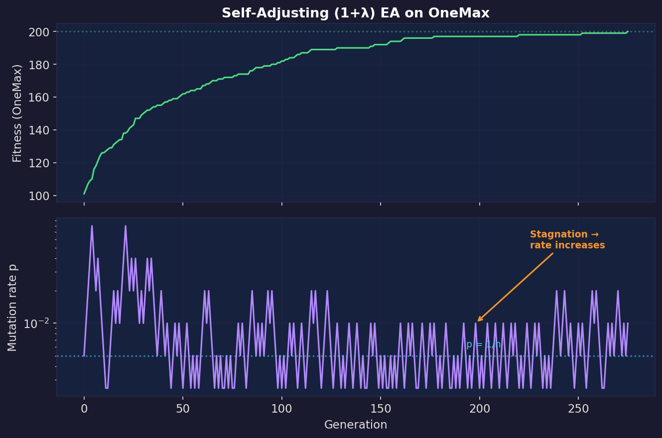
In practice: when progress is possible with small perturbations, the process drifts towards smaller mutation rates (exploitation). When it gets stuck, larger rates win the offspring tournament, so the algorithm inflates its mutation rate (exploration). This is what we were doing heuristically on Rastrigin with the decaying $\sigma$ schedule, except that self-adjustment is data-driven and provably near-optimal.
Mapping the Rastrigin experiments to the theory
The Rastrigin GIFs are continuous and the theorems above are mostly discrete, but the lesson transfers because the failure modes are the same.
| Scenario | Elitism | Ergodicity | Selection | Outcome |
|---|---|---|---|---|
| Too little diversity | Yes | Technically, but $\sigma$ too small | Very strong | Local optimum |
| Too much diversity | Yes | Yes | Too weak | Random walk |
| Balanced diversity | Yes | Yes | Moderate | Global optimum |
Too little diversity. Rudolph’s convergence conditions are met (elitism is on, Gaussian noise is ergodic), so convergence is guaranteed in theory. But the takeover curves show why it’s useless in practice: strong selection collapses the population in $\Theta(n \log n)$ iterations, and once diversity is gone, escaping the local optimum requires an exponentially unlikely mutation (Dang et al.).
Too much diversity. Weak selection can’t compound improvements, so the population wanders without exploiting what it finds.
Balanced. The population starts diverse (enabling the polynomial escape time from Dang et al.) and gradually focuses as the mutation schedule decays (approximating the self-adjusting strategy from Doerr et al.).
The recipe:
- Use elitism so “discovering the best-so-far” is sticky.
- Keep selection pressure moderate so takeover doesn’t annihilate diversity immediately.
- Set mutation strength near the optimum ($c \approx 1$ in the discrete case, or the equivalent $\sigma$ in continuous problems), since the runtime cost of overshooting grows rapidly.
- If you have recombination, make sure the population stays meaningfully diverse. Otherwise crossover is provably wasted on difficult landscapes.
- Prefer adaptive schemes when you can, because simple self-adjustment can track near-optimal settings on the fly.
The point
Evolutionary algorithms are not random search, and they have provable convergence guarantees, but those guarantees are vacuous without diversity management. Too little diversity and you’re stuck; too much and you’re lost. The science is in controlling the transition from exploration to exploitation as the algorithm runs.
All code to generate the animations and figures in this post is available at github.com/GeometricAGI/blog.
References
-
G. Rudolph. Convergence Analysis of Canonical Genetic Algorithms. IEEE Transactions on Neural Networks, 5(1):96-101, 1994. doi:10.1109/72.265964
-
G. Rudolph. Takeover Times and Probabilities of Non-Generational Selection Rules. In Proceedings of the Genetic and Evolutionary Computation Conference (GECCO), pp. 903-910, 2000.
-
D.E. Goldberg and K. Deb. A Comparative Analysis of Selection Schemes Used in Genetic Algorithms. Foundations of Genetic Algorithms, 1:69-93, 1991.
-
C. Witt. Tight Bounds on the Optimization Time of a Randomized Search Heuristic on Linear Functions. Combinatorics, Probability and Computing, 22(2):294-318, 2013. doi:10.1017/S0963548312000600
-
D.-C. Dang, T. Friedrich, M. Kötzing, M.S. Krejca, P.K. Lehre, P.S. Oliveto, D. Sudholt, A.M. Sutton. Escaping Local Optima with Diversity Mechanisms and Crossover. GECCO 2016, pp. 645-652. doi:10.1145/2908812.2908956
-
D.-C. Dang, T. Friedrich, M. Kötzing, M.S. Krejca, P.K. Lehre, P.S. Oliveto, D. Sudholt, A.M. Sutton. Escaping Local Optima using Crossover with Emergent Diversity. IEEE Transactions on Evolutionary Computation, 22(3):484-497, 2018. doi:10.1109/TEVC.2017.2724201
-
B. Doerr, C. Gießen, C. Witt, J. Yang. The (1+λ) Evolutionary Algorithm with Self-Adjusting Mutation Rate. Algorithmica, 81:593-631, 2019. doi:10.1007/s00453-018-0502-x
-
D. Sudholt. The Benefits of Population Diversity in Evolutionary Algorithms: A Survey of Rigorous Runtime Analyses. arXiv:1801.10087, 2018.
-
T. Friedrich, P.S. Oliveto, D. Sudholt, C. Witt. Analysis of Diversity-Preserving Mechanisms for Global Exploration. Evolutionary Computation, 17(4):455-476, 2009. doi:10.1162/evco.2009.17.4.17401